User guide for decadal forecasts

Introduction

This guidance document describes how to access and use multi-model ensembles of decadal forecasts for Canada served by Canadian climate data and scenarios (CCDS). This document outlines the key features and factors to consider when using the decadal forecasts for Canada. A technical document for the decadal forecasts is also available.

What is a decadal forecast?

Decadal forecasts bridge the gap between seasonal forecasts and climate projections. They can support decision-making by providing users with near-term predictions up to 10 years into the future. Decadal forecasts are produced by initializing complex Earth system models with current observed climate conditions and running them forward for up to a decade. A similar product that provides near-term forecasts is seasonal forecasts. However, seasonal forecasts, such as those available on CCDS, only forecast monthly and seasonal changes from 1 to 12 months into the future. Both types of datasets can help predict the likelihood of climate variables, such as temperature or precipitation, to deviate from recent climate conditions.

How should decadal forecasts be used?

Decadal forecasts can help users understand climatic changes in the near-term future, spanning 1–10 years. They should be used when regional climate predictions are needed for the coming decade, beyond the period available in seasonal forecasts.

Why use a decadal forecast?

The decadal forecasts on CCDS describe the difference relative to average conditions during a reference period. They are predicted by global modelling centres for variables such as temperature and precipitation. These differences are known as climate anomalies. Climate anomalies are useful for highlighting predicted local changes in comparison to historical observations. The decadal forecasts on CCDS consist of multi-model ensembles for each season and the entire year.

Seasonally specific forecasts can inform local policies and highlight potential climatic shifts in Canada’s seasons. Compared to absolute forecasts, forecasts using anomalies can provide users with the predicted magnitude of change. This often offers more context for decision-making.

When not to use a decadal forecast?

Decadal forecasts are not available beyond 10 years into the future. Users can acquire this information by consulting long-term climate projections produced by global modelling centres.

The decadal forecasts on CCDS describe predicted conditions averaged over the year or a season. The upper (95^th percentile) and lower (5^th percentile) percentiles of decadal forecasts describe the range of these predictions across models. However, these forecasts do not provide information about extremes within a year or season.

Other derived products available on CCDS, such as climate extreme indices, are more suitable options to support these types of analyses. Please refer to the CCDS site overview for a list of available datasets.

Climatology for the forecasted anomalies across Canada

Anomalies are calculated using a climatology period (also known as a reference period). Climatology refers to the average conditions over a period, typically spanning 30 years.

The ensemble datasets for Canada on CCDS use anomalies calculated by the World Meteorological Organization (WMO) Lead Centre for Annual to Decadal Climate Prediction (WMOLC). The 1991 – 2020 climatology period is used to reflect recent climate conditions. Anomalies that use an older climatology period will predict results with different magnitudes. This can be useful for individuals who manage long-lived infrastructure products. However, the decadal forecasts presented on CCDS are meant to assess recent changes in climate across Canada.

Managing uncertainty

Types of uncertainty

Decadal forecasts, like weather predictions and climate projections, are naturally uncertain. This arises from uncertainty in initial conditions, from model limitations, and due to limits on predictability across a decadal timeline.

Uncertainty in each model’s initial conditions can arise from incomplete or imperfect observations of the current climate. This can impact the starting point for the forecast. Model limitations reflect the extent to which a model can accurately simulate complex climate processes. Limits on predictability over a decadal time scale are often due to the chaotic nature of the climate system. This is sometimes referred to as the “butterfly effect”. Uncertainty in future greenhouse gas emissions and other atmospheric changes can also reduce forecast accuracy over time. As the forecast period extends, predictions generally become less accurate.

How is uncertainty managed in the decadal forecasts?

Uncertainty in the decadal forecasts on CCDS is managed using two methods. First, multi-model ensembles are calculated from the modelled anomalies. Second, anomalies are averaged over rolling 5-year periods. For example, the forecasted anomaly for the summer of 2024–2028 is calculated as the average of the forecasted summer anomalies for a specific location over those 5 years. A similar procedure is carried out for 2025-2029, and so forth.

For more information on this process, please refer to the technical user document. This document contains information such as the model list, data processing methods, and steps for producing the percentile datasets.

Why was this method of uncertainty management used?

Uncertainty is managed using two methods, including a multi-model ensemble and a rolling average. Taking an ensemble of models provides a range of possible forecast outcomes for the next decade. The ensemble results are offered as percentiles, indicating how each forecast compares to the range of model predictions.

Forecasts for shorter intervals, such as a month or season within the next 5 to 10 years, are generally too uncertain to be useful. Large short-term variations, such as extreme temperature swings, are unpredictable and have a chaotic nature. They can mask long-term climate patterns, like ENSO cycles, which are generally more predictable. This is often referred to as “noise”. This “noise” is managed by calculating 5-year rolling averages on seasonal and annual forecasts. Calculating these rolling averages reduces the influence of unpredictable variations, providing a more stable forecast.

These methods cannot account for uncertainty due to incomplete knowledge of initial conditions. However, using a range of models can mitigate the limitations of any specific model. Smoothing out short-term fluctuations can emphasize underlying climate signals, highlighting predictable patterns in the climate over the forecast period.

Alternative methods to consider for managing uncertainty

The WMOLC uses skill maps to estimate the performance of each contributing model in their ensemble. Skill maps indicate a model's performance by showing how accurately it reproduces past conditions (hindcasting). Forecasts from models with low skill may have higher uncertainty and a lower chance of being correct for specific regions or variables.

Skill maps of the ensemble forecasts for Canada are not available on CCDS. However, global skill maps for the next 5-year forecast period are available on the WMO website.

Description of the global source datasets

The WMOLC and its annually issued Global Annual to Decadal Climate Update (GADCU) forecasts several variables. This includes global temperature and precipitation anomalies for the next five years (for example, 2024-2028). These forecasts are computed from monthly averaged forecast data across the globe, typically provided by 10-15 modelling centres.

The forecasts available on CCDS are from this ensemble of global climate models. For example, the ensemble for 2024-2033 includes the same 15 models for temperature and 14 models for precipitation used in the WMO’s 2024 report.

Each model produces a set of forecasts that start with unique initial conditions. Each of these forecasts is called a ‘run’ or ‘ensemble member’ of the model. Using multiple runs from a model helps account for uncertainty in initial conditions. All runs from a model are averaged and then masked to focus on the region of Canada. These model averages then contribute equally to the multi-model ensemble for Canada on CCDS.

All ensemble datasets for Canada are available as NetCDF files. NetCDF is a common file format in the field of climate science. NetCDFs can be read and processed with an array of programs such as Python, R, Climate Data Operators (CDO), ArcGIS, and MATLAB. For more information on these datasets, please refer to the technical user document.

Description of the output datasets for Canada

Percentiles of forecasted anomalies for Canada

Percentiles represent the threshold below which a certain percentage of data in a group falls. For Canada’s climate forecasts, the multi-model ensemble percentiles indicate the threshold below which a given percentage of models predict the forecasted anomaly.

For example, the 5^th percentile indicates a low-end outcome where only 5% of the models forecast anomalies at or below the presented value. Conversely, the 95^th percentile represents a high-end outcome, where 95% of the models forecast anomalies at or below the presented value. Thus, the 5^th and 95^th percentiles provide the approximate lower and upper bounds of predicted anomalies. The 50^th percentile marks the middle of the anomaly range, with half the models predicting higher values and half predicting lower values. Percentiles are an indicator of the range in uncertainty of forecasts from global modelling centres, offering flexibility in users’ analysis.

Annual and seasonal datasets of forecasted anomalies across Canada

Forecasted anomalies are available on annual and seasonal timescales, averaged across 5-year periods. All anomalies are relative to averages during the climatology period 1991-2020. Annual anomalies can provide an overview of yearly climate predictions, while seasonal anomalies can indicate predicted climate during the seasons. For example, seasonal forecasts predicting higher than average temperatures in one season versus another can help inform seasonally specific climate policy, which the annual forecasts cannot.

Maps of forecasted anomalies

Maps of forecasted anomalies across Canada illustrate how predicted climate variables compare to their reference period. They can indicate regional differences and can help support informed decision-making for the upcoming decade across Canada. Examples of forecast maps for temperature and precipitation are shown in Figures 1 and 2 below.

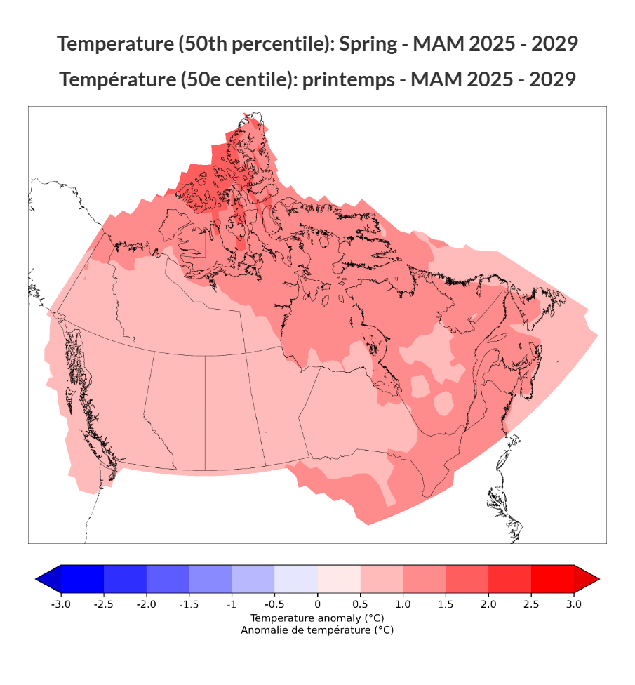
**Figure 1.** Temperature anomaly map of Canada for Spring 2025 – 2029, with anomalies greater than the baseline average shown in shades of red. Anomalies below the baseline average are shown as shades of blue but are not present in the figure.

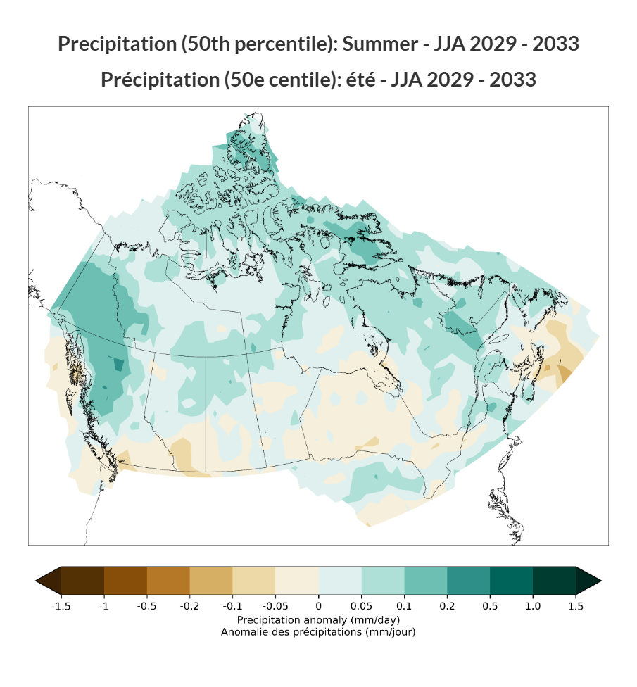
**Figure 2.** Precipitation anomaly map of Canada for Summer 2029 – 2033, with anomalies greater than the baseline shown in shades of green and anomalies below the baseline shown as shades of brown. For the precipitation maps on CCDS, a nonlinear scale was used to better capture the anomaly range from -1.5 to +1.5 mm/day.

Maps of the forecasted ensembles for Canada can be generated using the interactive webpage

For more information on the tools and the methods used for creating these datasets, please refer to the technical user document.

Accessing decadal forecasts on CCDS

The following section will guide the user in navigating the decadal forecast webpage. It will also explain some of the site’s components and provide an example of how to interpret the forecasts.

Downloading NetCDF datasets

Users can download NetCDF files of the ensemble forecasts for temperature and precipitation. To download these datasets from the CCDS webpage, use the menu on the side panel of the map. Select a variable, percentile, and time of year. The selection of the 5-year period will not affect the downloaded file. Once users have selected these options, they can click the “Download data as NetCDF” button located under the map to download the dataset.

Selecting point locations

Users can use the interactive map to compare local forecasted anomalies for up to 10 different locations across Canada. To add a new marker to the map, choose the “Add Marker” button under the side panel menu. With the new marker selected, there are two options to select a location:

Search for cities across Canada using the search bar located under the map. The marker name will update to reflect the city selected from the search bar
Alternatively, the user can scan the interactive map with their cursor to find specific coordinates. The coordinates over which the cursor hovers update continuously below the map. Double-click the location of interest on the map to include the location in the “Selected markers” panel. Update the name of this location using the rename button located in the side panel associated with the marker. User-defined names will reset if a new location is selected for that marker

All selected locations, either through the search bar or by scanning the interactive map, will show in the side “Selected markers” panel. Each point will have a unique pop-up on the map displaying the point name, the coordinates, and the anomaly value for that variable. The anomaly will update as menu options for the map are changed.

Saving map plots

Once locations of interest have been selected and desired menu options have been applied, PNG images of the generated map can be downloaded. There is the option to download the map with or without markers by clicking one of the “download map…” buttons located below the map.

Comparing ensemble percentiles at selected locations

Different ensemble percentiles of forecasted anomalies can be compared across the selected locations listed in the “Selected markers” panel. A table at the bottom of the page is automatically generated. The table lists the location names with their nearest coordinates on the 1x1-degree grid and the anomalies for all 5 percentiles. This table will update dynamically when the menu selections change in the side panel. It provides a quick overview of the spread in the forecasted anomalies across the user-selected locations. Users can download tabulated results as a CSV file by selecting the “download table as CSV” button located below the table.

Example

This brief example will guide users through a visual analysis of forecasted precipitation. The objective of this example is to download and compare the 50^th percentile of 5-year annual and seasonal precipitation across Canada. This example will focus on the 2027 – 2031 period.

On the ‘Decadal Forecast for Canada’ webpage, the user should first apply the appropriate menu selections. For this example, the variable is “precipitation”, the ensemble percentile is “50th percentile”, and the time period is “2027-2031”. This analysis will compare the annual forecasted precipitation anomalies to the anomalies forecasted for each season. In this example, the city markers to select are: Ottawa, Ontario; Vancouver, British Columbia; and Thunder Bay, Ontario. Once selected using the methods outlined in the “Comparing different locations” section, select the “annual” time of year, and download the map with markers. The forecast map should look like Figure 3.

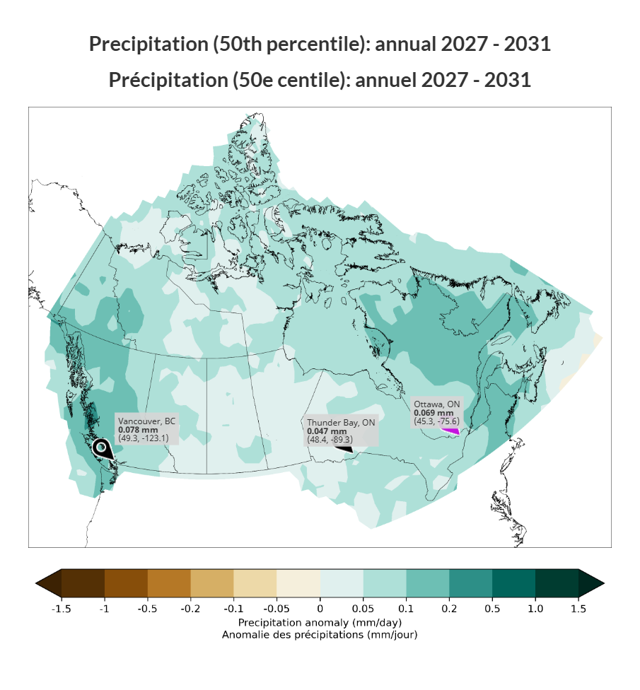
**Figure 3.** Map of the 50^th percentile of annual precipitation anomalies for Canada for 2027 – 2031.

Following similar methods, you can cycle through the other seasons in the “Time of Year” menu selection and download the maps for each season. The maps with markers should look like those presented in Figure 4a-d.

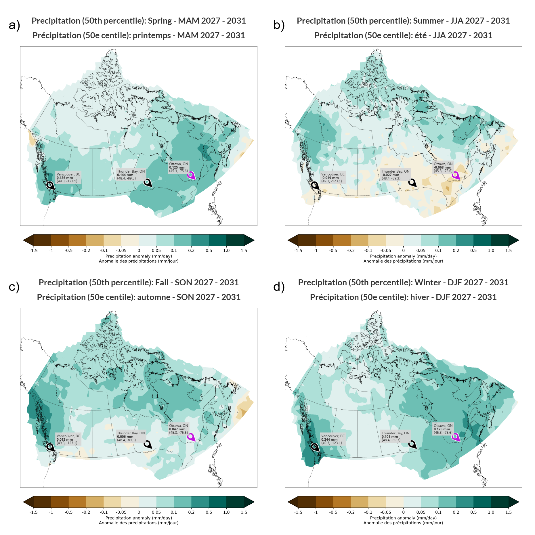
**Figure 4.** Maps presenting the 50^th percentile of precipitation anomalies for Canada: a) in spring, b) in summer, c) in fall, and d) in winter for 2027-2031.

Visually, we can see that the annual map displays similar anomaly patterns to the winter and spring maps. In these seasons, most locations across Canada predict wetter conditions than the 1991-2020 average. Wet anomalies are relatively low (light green) in interior provinces like Saskatchewan, Alberta, and Manitoba. Meanwhile, wetter conditions (darker green) are observed in areas like central Ontario, Quebec, and the Canadian coast. These observations imply that during the winter and spring, regions such as Ontario and Quebec may experience a greater change in average precipitation. In contrast, these same regions forecast fewer wet conditions in the summer and the autumn.

This contrast between seasons implies that a large amount of this region’s annually predicted increase in precipitation from 2027 to 2031 is expected to occur during the winter and spring. For central Ontario and Quebec, these two seasons act as primary drivers for the overall annual change in precipitation forecasted by the collection of models.

Dataset licence

Open Government Licence - Canada (http://open.canada.ca/en/open-government-licence-canada)

Individual model datasets and all related derived products, including the multi-model ensembles, are subject to the terms of use of the source organization.

Some of the contributing centers currently provide their data on open-source channels. For more information about a specific model, please contact the appropriate modelling center.

Contact

For additional support on the ensemble of forecasted anomalies for Canada, please contact ECCC using the following email: f.ccds.info-info.dscc.f@ec.gc.ca

If you have questions about the raw forecast data, please contact the WMO Lead Centre on the Annual to Decadal Climate Prediction. If you are interested in global information from the WMO Global Annual to Decadal Climate Update, please follow the link for the WMO’s report: WMO Global Annual to Decadal Climate Prediction (2024).

For answers to frequently asked questions, please visit the decadal forecast homepage on CCDS. Other inquiries can be sent to the previously listed email.

"Page details"

Date modified:: 2019-03-01